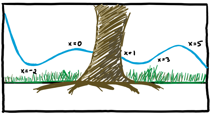

In the previous Monthly Math-y about finding roots, I talked about how to start with a (complicated) function and finding its horizontal intercepts by using numerical methods. I thought a good pairing for that is to discuss the reverse! In other words, building a function that passes through any number of points you desire. Passing through points is what we call ✨ Interpolation ✨.
What is so cool about this is that you're not relegated to just horizontal intercepts! You'll be able to pass through any collection of points you want, as long as you abide by one rule. You cannot repeat the same input! The main reason for this restriction is you never want to confuse the function on what it’s supposed to return as an output.
For example, suppose you have $(2,4)$ and $(2,5)$ where the first number in the parenthesis is the input and the second number is the output. Here we repeated the input “$2$”. When we ask for an output, we don’t know if we want $4$ or $5$ back!
This type of restriction is everywhere in the real world. Imagine if you sent a text message (the input) and the person receiving the message (the output) had two possibilities: your actual intended message or some jumbled mess of words. So, we want our data to be clear and non-confusing.
Let’s start! Suppose we have the data:
We have three points that we want our function to pass through. We start labeling with $x_0$ and $y_0$ because of convention. According to Wikipedia, the Lagrange Polynomial is the unique polynomial of lowest degree that interpolates a given set of data.
A polynomial is one of the simplest forms a function can be. You probably recognize $y = mx + b$ or maybe $y = ax^2 + bx + c$ which are both polynomials! Polynomials are functions where the only operations allowed are addition, subtraction, multiplication, and exponents with positive whole numbers! No divisions allowed, no negative exponents. You don’t really need to know that it’s unique, but it is cool that it is unique.
Degree refers to the largest exponent the variable of the polynomial has. So, “lowest degree” here means we don’t have to go up to a higher exponent to pass through all the points.
Heads up, I’m about to throw a huge math formula at you. The Lagrange Polynomial for the data $\{(x_0,y_0),(x_1,y_1),(x_2,y_2)\}$
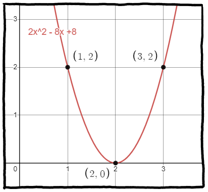
What I want to highlight about this is a few things. One, the polynomial we get will always have degree one less than the number of data points we have. For example, here we have three data points, and so our polynomial (after all the multiplying and simplifying) will look like $y = ax^2 + bx + c$. For completion of this example, the answer you would get is $2x^2-8x+8$ and looks like:

Two, this is a guaranteed process. As long your data abides by the one rule above, you will always find the Lagrange polynomial that can pass through those points. But there's a severe weakenss to this... We'll see it in the next section.
Three, this process is involved. There's a lot going on in terms of computing, so you can imagine what happens when there's 10 or 100 data points. If you had all the time and computing power, you could definitely find a lot of Lagrange Polynomials for what data set you have. There's also the limit that this only works for two-dimensional data! You can only have $(x,y)$'s. (There's actually higher dimensional versions, but that's outside my pay grade.)
That brings up a good question (and segue to the next topic), what do we do if don't have the strongest computer to do 10 or 100 data points just to find one polynomial?
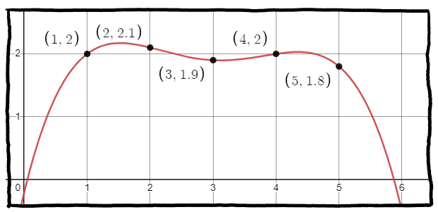
Why exactly are we making polynomials that passes through points? (Besides that it's cool we can do this.) We want to estimate! We have a data set and what we really want is to know what happens outside of that data, maybe to guess what will happen in the future. So, the weakness I alluded to above can be seen in the following sketch:

What happens when we want to estimate what happens at input 6? Well, we've fallen into the negatives! But, by inspection, the data seems to float around the height of 2. The issue here is that the Lagrange polynomial is too exact with its data, but outside of that data, we're probably not doing a great job at finding the "trend" or "pattern".
For this example, the "line of best fit" is probably the horizontal line at height 2. Sure, it messes up the other values, but at least it has the correct trend. The line of best fit also has the fancy name of "linear regression" which you can watch a video demonstrating it, but this is already outside what I wanted for this Monthly Math-y. The idea is that we're finding a line (or curve) that has the "least square error" which is another fancy thing that I might talk about in a future Monthly Math-y.
So, why did I bring up this topic? (Besides that it's cool.) I wanted to highlight this weird thing about mathematics and our needs in the real-world, what appears to be a dichotomy (a division or contrast between two things that are or are represented as being opposed or entirely different.) On one hand, you have a mathematically sound process that will do exactly what you want it to do (give you a polynomial that passes through a set of data points). On the other hand, the real world needs things that we can do efficiently, even if it means there will be an error.
What I want to argue is that these two avenues aren't so opposing. There are probably other parts of mathematics where this sort of dichotomy exists between pure curiousity and applied needs. It most certainly is a dichotomy that some mathematicians find themselves believing can never be remedied. As someone who has been on both camps, it really does not seem all that different. At the end of the day, what I believe to be mathematics is understanding our world and what we, humans, can do with our creations/discoveries. I think people on both sides ought to appreciate that the other camp exists to do the thing that you may not want to do. The proof of the Lagrange polynomial being unique, or that it even exists, can be tiresome, but someone who loved the venture of mathematics found it fulfilling to do. Now we have it. Similarly, the discovery of the least squares error line of best fit is something that took years to find and implement for computers. But now we have it.
Uploaded 2023 August 1. (This was added to the ordering afterwards to complete a year-long collection.) This is a part of a monthly project which you can read about here.